Training a YOLOv26 Model for 3D Print Failure Detection
Train a custom YOLOv26 model to detect spaghetti, stringing, and zits in 3D prints. From a failed first dataset to a 0.98 mAP spaghetti detector trained on the cloud for under $2.
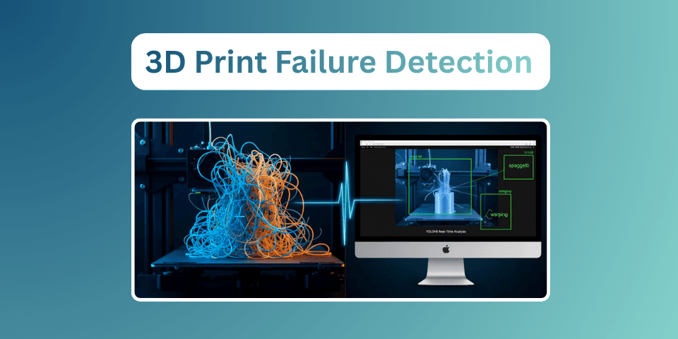
Why Automate Failure Detection?
Watching a 3d print (for hours) is one of my favorite pastimes. However, it's not always possible. Especially when prints run for three days at a row. Biggest risk is that you fall asleep at 2 AM, while a 48 hour print slowly turns into a plate of spaghetti. The problem with manual monitoring:
- You can't watch 24/7. Multi-day prints run overnight, during work, during life.
- By the time you notice, it's too late. A spaghetti failure at hour 30 means 30 hours of wasted time and filament.
- Filament isn't cheap. At about ₹1,000 per kg, a failed 200g print wastes real money.
- Unattended failures are a fire risk. A detached print can hit the nozzle, melt, and cause serious problems.
What if the webcam could think? What if it could recognize when a print is failing and either alert you or stop the printer automatically?
That's exactly what we're building: a YOLOv26-based object detection pipeline that watches your printer through a webcam, detects common failure modes, and takes action. This post covers the first half - training the model. In Part 5, we'll build the real-time monitoring script and automated printer control.
The Pipeline Architecture
Here's what the complete system looks like:
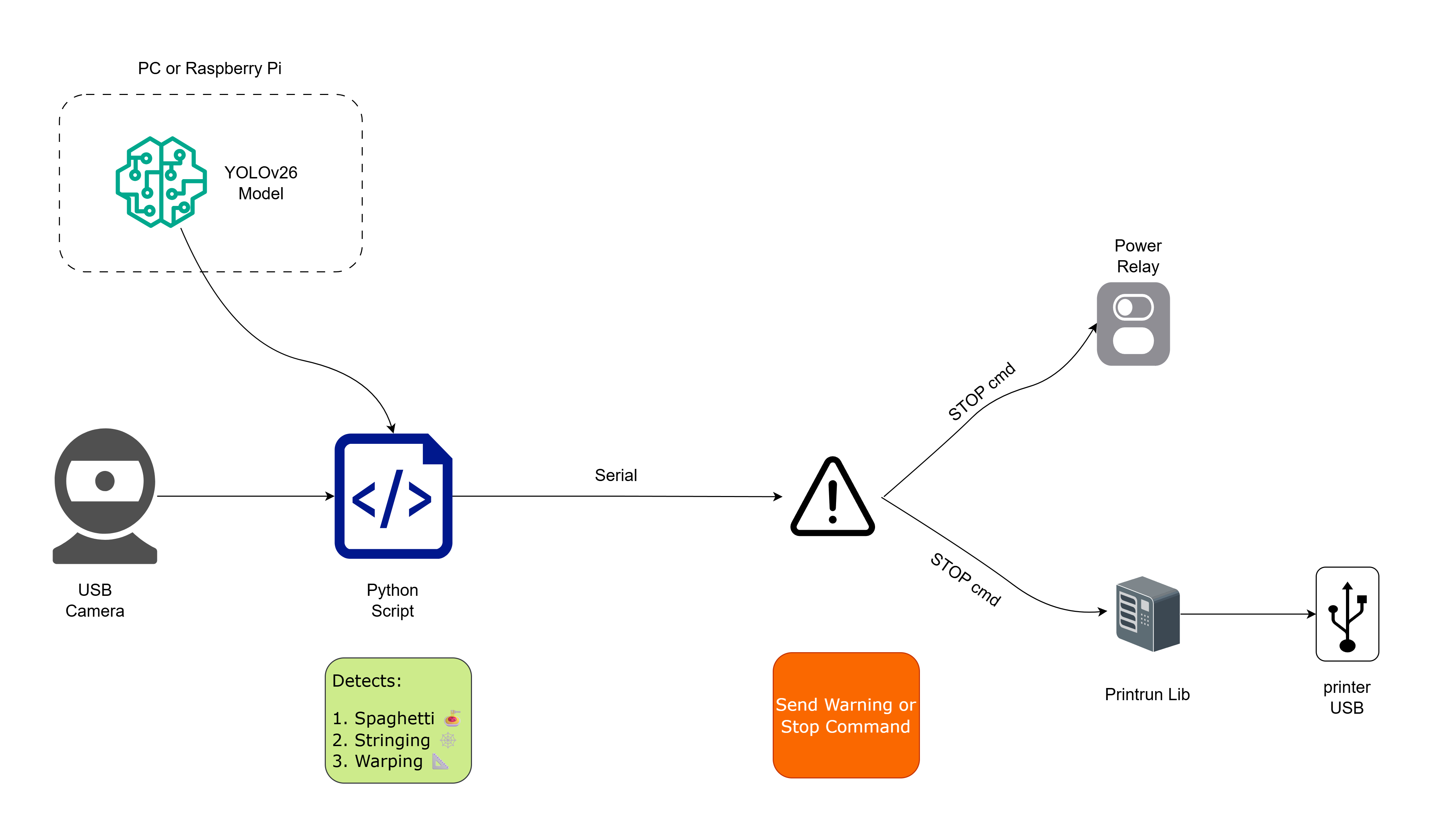
Three components:
- YOLOv26 Model : Trained on annotated images of 3D print failures from Roboflow (this post)
- Monitoring Script : Captures webcam frames, runs inference, detects failures (Part 5)
- Action Layer : Sends alerts (Telegram, email) and/or stops the printer via G-code (Part 5)
Setting Up the Environment
You'll need Python 3.8+ and a few packages:
1# Create a virtual environment (recommended)
2python -m venv print_detect_env
3source print_detect_env/bin/activate  # Linux/macOS
4# print_detect_env\Scripts\activate  # Windows
5
6# Install dependencies
7pip install ultralytics roboflow opencv-python
Hardware notes:
- Training: A GPU is strongly recommended. An NVIDIA GPU with 6GB+ VRAM works for 640px images. For higher resolutions (1024px), you'll want 24GB VRAM , or use a cloud GPU.
- Inference: CPU is fine for real-time webcam monitoring at 1-2 FPS, which is more than enough for print failure detection. You don't need 30 FPS here : prints fail over minutes, not milliseconds.
The Training Journey
What follows is the full experiment log , including the dead ends. I'm keeping the failed attempts in because they taught me more than the successful ones.
Experiment 1 , The Wrong Dataset (Local, RTX 3060 12GB)
I started with this dataset from Roboflow Universe , about 4,500 images with three classes:
| Class | What It Looks Like | Severity |
|---|---|---|
| Spaghetti | Filament going everywhere, print detached from bed | 🔴 Critical : stop immediately |
| Stringing | Fine strands of plastic between parts | 🟡 Warning : may self-correct |
| Warping | Corners lifting from the bed | 🟠 Moderate : likely to get worse |
Looked great on paper. Downloaded it in YOLO format:
1from roboflow import Roboflow
2
3# Initialize with your API key
4rf = Roboflow(api_key="YOUR_API_KEY")
5
6# Access the dataset
7project = rf.workspace("bigvision-iwppy").project("3d-print-failure-detection-efvsh-cewsr")
8version = project.version(1)
9
10# Download in YOLOv26 format
11dataset = version.download("YOLOv26")
This creates a folder structure like:
13d-print-failure-detection-1/
2├── data.yaml          # Dataset config (class names, paths)
3├── train/
4│   ├── images/        # Training images
5│   └── labels/        # YOLO format annotations
6├── valid/
7│   ├── images/
8│   └── labels/
9└── test/
10    ├── images/
11    └── labels/
Trained the standard way , YOLO26 nano, 50 epochs, 640px:
1from ultralytics import YOLO
2
3model = YOLO("yolo26n.pt")
4
5results = model.train(
6    data="3d-print-failure-detection-1/data.yaml",
7    epochs=50,
8    imgsz=640,
9    batch=16,
10    name="print_failure_detector",
11    patience=10,
12    save=True,
13    plots=True,
14)
The results were bad:
| Run | Model | Epochs | mAP50 | Notes |
|---|---|---|---|---|
| v8 nano | YOLOv8n | 50 | 0.225 | Plateaued immediately |
| v8 medium | YOLOv8m | 50 | 0.220 | Larger model didn't help |
| v26 nano | YOLO26n | 50 | 0.225 | New architecture, same ceiling |
| v26 small | YOLO26s | 150 | 0.258 | More epochs, marginal gain |
mAP50 plateaued at ~0.25 regardless of model size, architecture, or training duration. I tried everything , longer training, bigger models, different learning rates. Nothing moved the needle.
Then I looked at the labels. Plotted bounding boxes on random training samples and found widespread problems: normal prints labeled as "spaghetti", layer lines labeled as defects, overlapping/redundant boxes on the same object. The dataset looked fine on paper (4,500 images, 3 classes) but had serious annotation quality issues.
Lesson learned: Always visually inspect your dataset before trusting the numbers. A model can only be as good as its labels.
Experiment 2 , Clean Data Changes Everything (Local, RTX 3060 12GB)
Switched to a much better-annotated dataset: 3D Printing Failure , about 9,000 images with 43,500+ bounding boxes. This dataset has different classes:
| Class | What It Looks Like | Severity |
|---|---|---|
| Spaghetti | Filament going everywhere, print detached from bed | 🔴 Critical : stop immediately |
| Stringing | Fine strands of plastic between parts | 🟡 Warning : may self-correct |
| Zits | Small blobs/bumps on the print surface | 🟢 Minor : cosmetic defect |
I'm not overly concerned about zits , they're cosmetic and don't threaten the print. Spaghetti is the one that matters. It means the print has completely detached and is creating a tangled mess. That's the detection that needs to be near-perfect. I went with this dataset because its spaghetti annotations were clean and plentiful.
1from roboflow import Roboflow
2
3rf = Roboflow(api_key="YOUR_API_KEY")
4
5project = rf.workspace("3d-printing-failure").project("3d-printing-failure")
6version = project.version(1)
7
8dataset = version.download("YOLOv26")
Same YOLO26 nano model, same 640px, same machine. The results were night and day:
| Run | imgsz | Batch | Epochs | mAP50 | Notes |
|---|---|---|---|---|---|
| nano (640px) | 640 | 8 | 50 | 0.622 | 3x improvement over Experiment 1 |
| nano (800px) | 800 | 16 | 70+ | 0.697 | Higher res helped small defects |
The same YOLO26n architecture went from 0.225 → 0.622 mAP50 just by switching to a properly-labeled dataset. That's a 3x gain. Data quality was the bottleneck all along.
Bumping the image size from 640 to 800px also helped , especially for zits, which are tiny and need more pixel density to be visible to the model. But the loss was still decreasing at epoch 50; the model clearly needed more training time and my 12GB RTX 3060 was limiting batch sizes at higher resolutions.
Experiment 3 , Cloud GPU Training (RunPod, RTX 4090 24GB) ⭐
Time to throw proper hardware at this. I rented an RTX 4090 (24GB VRAM) on RunPod for $0.59/hr. The extra VRAM let me push to 1024px image size with batch=32 , both impossible on my local 12GB card.
[!TIP] RunPod gives you free credits on first signup , enough for a training run or two. Even without free credits, a full 100-epoch run cost me about $2 total. That's ridiculously cheap for the compute you get.
Training config:
1from ultralytics import YOLO
2
3model = YOLO("yolo26n.pt")
4
5model.train(
6    data="3D-printing-failure-1/data.yaml",
7    imgsz=1024, batch=32, epochs=100,
8    name="print_failure_detector_v26_nano_4090",
9    cos_lr=True, patience=20,
10    box=8.5, cls=1.0,               # boosted box loss weight
11    mosaic=1.0, close_mosaic=15,     # mosaic augmentation
12    mixup=0.15, copy_paste=0.15,     # instance-level augmentation
13    scale=0.7, degrees=10.0,         # geometric augmentation
14    shear=2.0, flipud=0.1,
15    erasing=0.3,                     # random erasing
16    hsv_h=0.02, hsv_s=0.75, hsv_v=0.5,  # color jitter
17)
A few things worth noting about this config:
box=8.5, I boosted the box loss weight significantly. The default is 7.5. Since spaghetti and stringing have irregular shapes, making the model try harder on localization helps.cos_lr=True, Cosine learning rate decay gives a gentler cooldown than step decay, which I found helped in the later epochs.close_mosaic=15, Mosaic augmentation is powerful for small object detection, but turning it off for the final 15 epochs lets the model fine-tune on clean, undistorted images.copy_paste=0.15, mixup=0.15, Instance-level augmentations help the model generalize across different print setups, camera angles, and lighting conditions.
Training took 2 hours 45 minutes , vs. what would have been 5+ hours locally (and at lower resolution).
Training Results
Loss and Metrics Over 100 Epochs
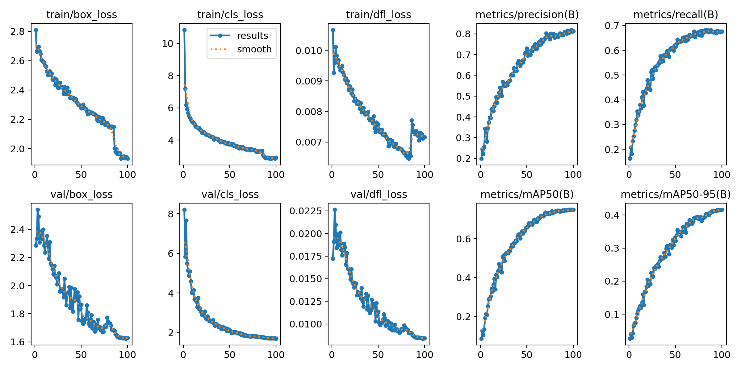
Both training and validation losses decreased steadily throughout training. The mAP50 curve (bottom right) shows a clean, monotonic climb from ~0.09 at epoch 1 to 0.749 at epoch 100, with no signs of overfitting. The model could likely benefit from more epochs, but the gains were flattening.
Final Model Performance
| Class | Precision | Recall | mAP50 | mAP50-95 |
|---|---|---|---|---|
| All classes | 0.812 | 0.678 | 0.749 | 0.416 |
| 🍝 Spaghetti | 0.937 | 0.947 | 0.980 | 0.670 |
| 🧵 Stringing | 0.778 | 0.669 | 0.743 | 0.380 |
| 🔵 Zits | 0.720 | 0.419 | 0.524 | 0.198 |
The numbers that matter most: spaghetti detection is at 0.98 mAP50 with 94.7% recall. That means the model catches nearly every spaghetti failure , which is the critical defect that can waste hours of filament and potentially damage the printer. This is exactly what we need for the monitoring system in Part 5.
Stringing sits at a solid 0.743 mAP50 , good enough to alert but not so critical that we need perfection. Zits at 0.524 is the weakest class, which makes sense , they're tiny surface blobs that are inherently hard to detect, and we can live with lower recall on a cosmetic defect.
Inference speed: 1.0ms/image on RTX 4090 (1000 FPS). For our monitoring use case at 1 FPS, even a CPU is overkill.
Model size: 5.5MB (2.5M parameters, 5.8 GFLOPs). Tiny enough to run on a Raspberry Pi.
Precision-Recall Curves
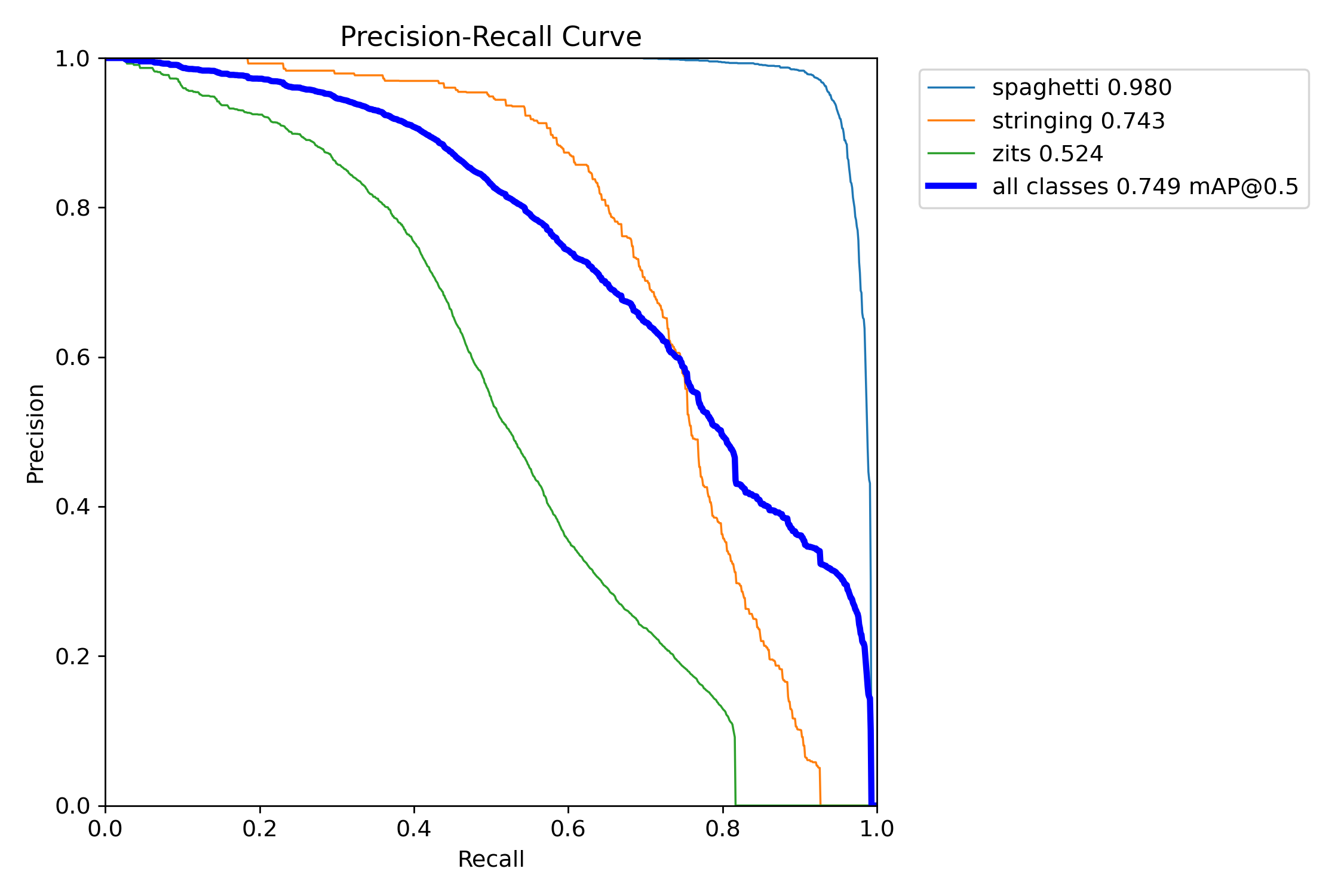
The PR curve tells the story clearly , spaghetti (light blue) maintains near-perfect precision even at very high recall. The model barely makes mistakes on the class that matters most. Stringing and zits trade off precision for recall more aggressively, which is expected given the nature of those defects.
F1-Confidence Curve
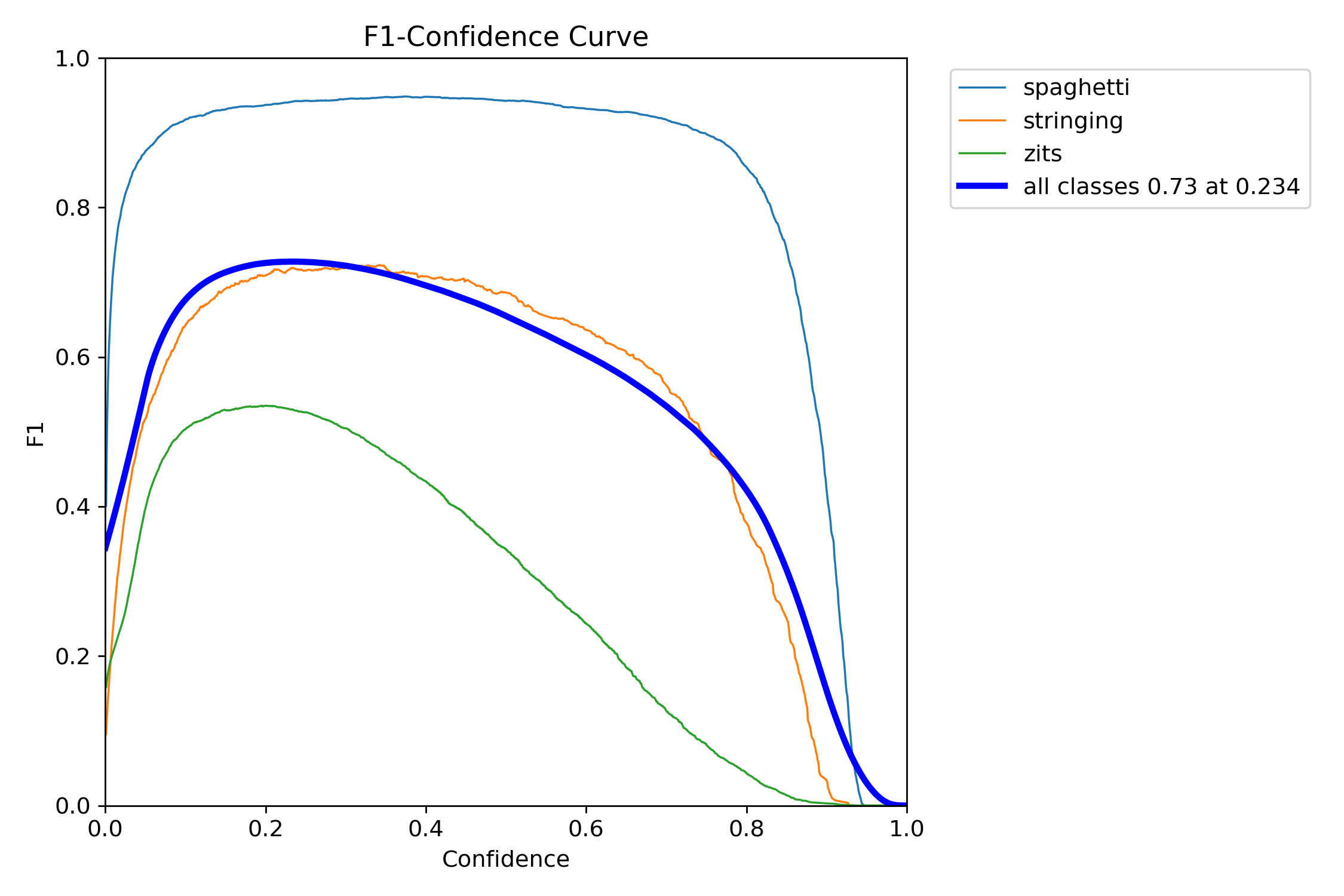
The F1-Confidence curve shows the optimal confidence threshold is around 0.234 for maximum overall F1 (0.73). In practice, for the monitoring system, I use a higher threshold of 0.5 to reduce false alarms , trading a bit of recall for fewer "your print is failing!" alerts when nothing is actually wrong.
Notice how spaghetti (light blue) maintains a high F1 score across almost the entire confidence range , even at 0.8 confidence, you're still catching most spaghetti failures. That gives us a lot of room to tune the threshold.
Confusion Matrix
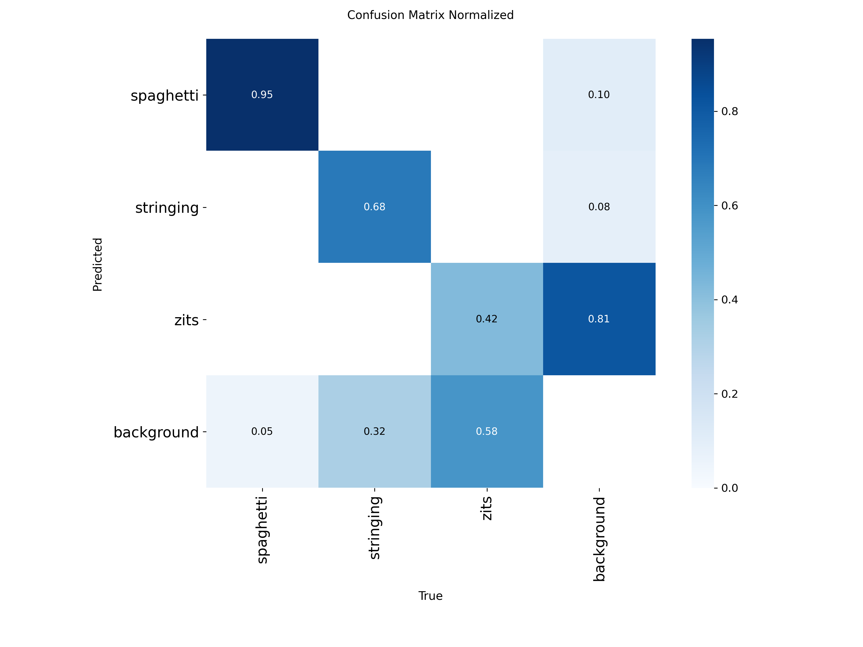
The confusion matrix reveals interesting patterns:
- Spaghetti: 95% correctly detected, only 5% missed as background. Almost no confusion with other classes.
- Stringing: 68% correctly detected, 32% missed as background. Some stringing is genuinely subtle , thin wisps that even humans might miss at certain angles.
- Zits: 42% correctly detected, 58% missed as background, with 81% of background regions falsely flagged as zits. This is the hardest class , zits are tiny, numerous (31K+ annotations), and can look like normal surface texture at low resolution.
Dataset Distribution
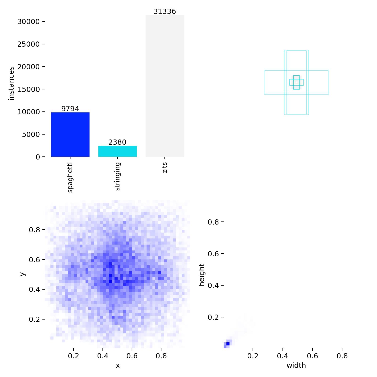
The dataset is heavily imbalanced , zits dominate with 31,336 annotations (72%) vs. spaghetti at 9,794 (22.5%) and stringing at 2,380 (5.5%). The bounding box size distribution (top right) confirms what we see in the metrics: zits boxes are tiny (clustered at tiny widths and heights), while spaghetti and stringing boxes are larger and more varied.
Validation Predictions
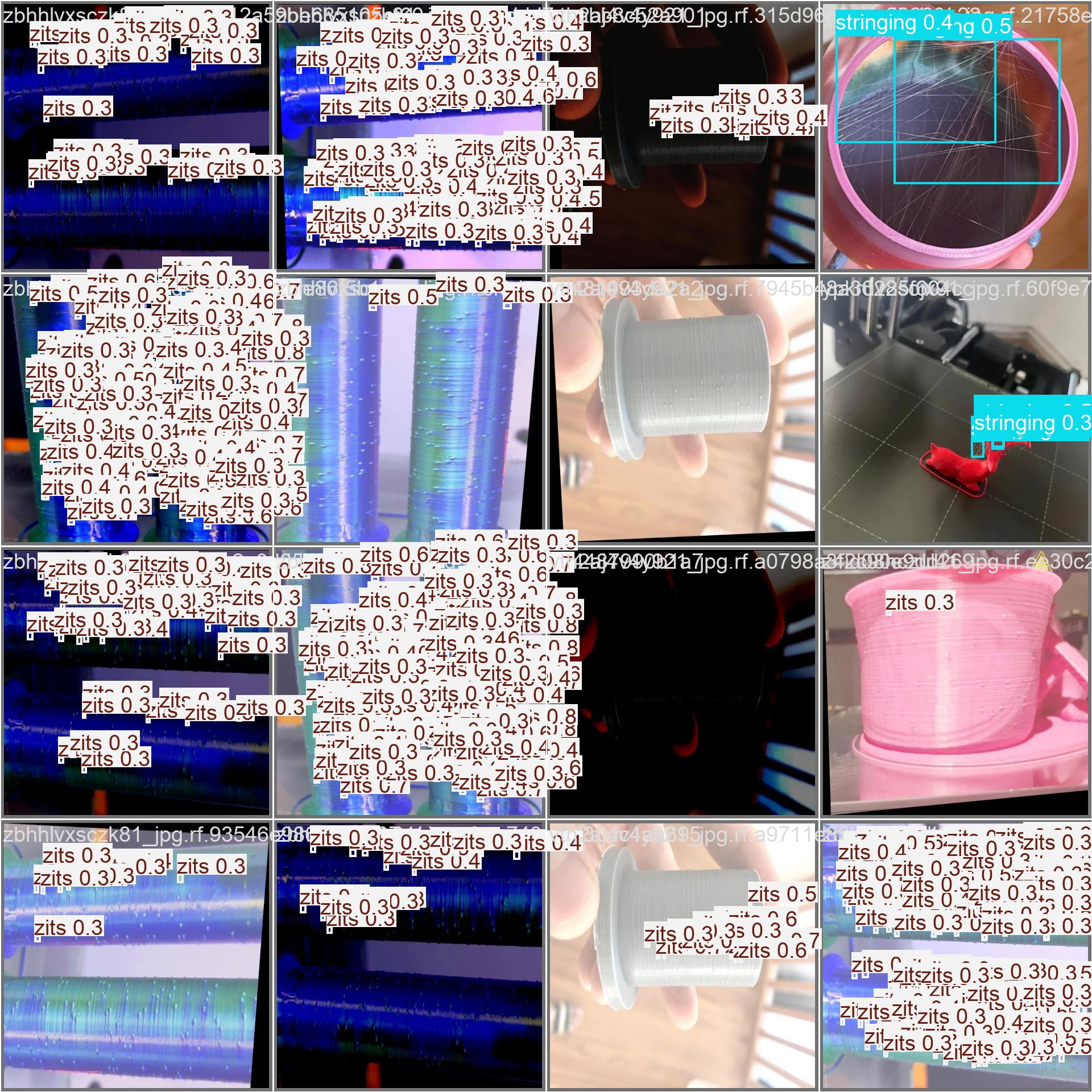
Here's the model running on unseen validation images. You can see it detecting zits and stringing with appropriate confidence scores. The model handles diverse lighting conditions, camera angles, and print materials , exactly what we need for a real-world monitoring system.
Results Summary Across All Experiments
1mAP50 progression:
2
3Exp 1 , bad dataset, 640px:   █████░░░░░░░░░░░░░░░░░░░░░░░░░  0.225
4Exp 2 , clean data, 640px:    ████████████████████░░░░░░░░░░░  0.622
5Exp 2 , clean data, 800px:    █████████████████████░░░░░░░░░░  0.697
6Exp 3 , clean data, 1024px:   ██████████████████████░░░░░░░░░  0.749
7                              ──────────────────────────────→
8                              0.0                         1.0
Key Takeaways
-
Dataset quality >> model size >> training time. Switching from a poorly-labeled 4,500-image dataset to a well-labeled 9,000-image dataset improved mAP50 from 0.225 → 0.622 , a 3x gain with the exact same model architecture. No amount of hyperparameter tuning can fix bad labels.
-
Input resolution is the #1 lever for small objects. 640 → 1024px improved zits detection (mAP50 0.370 → 0.524) because the model can actually see the tiny dots. If you're detecting small defects, push the resolution up as far as your VRAM allows.
-
YOLO26n (nano) is plenty for this task. 2.5M params achieved 0.98 mAP50 on spaghetti , the critical defect. I tried scaling to YOLO26s and YOLO26m with no meaningful improvement. Save the compute.
-
Always visually inspect your labels. The first dataset looked fine on paper (4,500 images, 3 classes) but had widespread mislabeling. The only way to catch this was plotting bounding boxes on random samples. I wrote a small viewer script for this , it's worth the 30 minutes.
-
Cloud GPU is ridiculously cost-effective. A full 100-epoch training run on RTX 4090 cost about $2 total and completed in under 3 hours vs. 5+ hours locally at lower resolution. RunPod even gives free credits on first signup.
Inference Performance on Different Hardware
One important consideration is where you'll actually run this model. Training requires a GPU, but inference (running the model on live frames) can work on much more modest hardware. Here's what I tested:
| Hardware | Model | Inference Time (per frame) | FPS | Practical? |
|---|---|---|---|---|
| RTX 4090 (Cloud) | YOLO26n | ~1ms | ~1000 | ✅ Way overkill |
| RTX 3060 (PC) | YOLO26n | ~8-12ms | ~80+ | ✅ Overkill for this task |
| RTX 3060 (PC) | YOLO26s | ~15-20ms | ~50+ | ✅ Also overkill |
| Intel i7 CPU (PC) | YOLO26n | ~80-120ms | ~8-12 | ✅ More than enough |
| Raspberry Pi 4 (4GB) | YOLO26n | ~1.5-2.5s | ~0.4-0.7 | ✅ Usable - 1 frame every 2-3s |
| Raspberry Pi 4 (4GB) | YOLO26s | ~4-6s | ~0.15-0.25 | ⚠️ Slow but functional |
[!NOTE] These benchmarks are approximate and depend on image resolution, background processes, and thermal throttling (especially on the Pi). Your results may vary - but the relative performance differences hold.
What's Next?
The model is trained and ready. In Part 5, we'll build the complete monitoring pipeline - connecting the model to a live webcam feed, implementing alert notifications, and automating printer control to stop prints when failures are detected.
Full Code Reference
The complete training notebooks and scripts from this post are available here: 3D Print Failure Detection.
Series Navigation:
- Getting Started with the Ender 3 V2 Neo
- Calibrations That Actually Matter
- Slicer Deep Dive & Long Print Survival
- AI Print Failure Detection - Training YOLOv26 (You are here)
- Real-Time Print Monitoring & Automated Control
Resources:
Previous Post
YOLOv26 Breakdown: NMS-Free Detection Meets LLM-Inspired Training
Next Post
Building a Real-Time 3D Print Monitoring System with YOLOv26
If the article helped you in some way, consider giving it a like. This will mean a lot to me. You can download the code related to the post using the download button below.
If you see any bug, have a question for me, or would like to provide feedback, please drop a comment below.